“Animals do not care about the evolution of the universe. Nor do many humans.”
— Stephen Hawking —
In this chapter, we will show how to create a computer model of a galaxy in order to study galaxy dynamics. The creation of initial conditions for galaxies is some kind of black magic. A century ago, nobody even knew that galaxies exist. The Milky Way galaxy and the universe were synonymous. Now, astronomers believe that galaxies mainly contain the matter of form other than we know from our everyday life.
A galaxy is a massive ensemble of stars and other material orbiting about a common center and its constituents held together by the mutual gravitational interaction. Galaxies come in the variety of global shapes and internal morphologies. They can be, however, broadly classified into two major types: elliptical and disk galaxies.
To our understanding, before the formation of first galaxies were in the universe immense shapeless low-density diffuse clouds of light elements. Due to gravity, they started to contract and collapsed into smaller fragments of the size of galaxies. During runaway gravitational collapse, where stars formed quickly in large numbers and started to shine at once before the gravitational collapse finished, an elliptical protogalaxy was born. The energy of gravitational collapse was not lost (dissipationless collapse) and was converted to the chaotic motion of stars. If the primordial gas was shrunken by the gravity more slowly, the gas have had enough time to start rotation and settled into a regular disk galaxy where it formed stars. Galaxy’s appearance therefore mirrors its formation. This is known as the gravitational collapse theory of a galaxy formation. In Chapter 6 will be shown that a subsequent evolution is important as well.
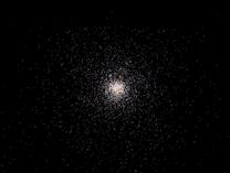
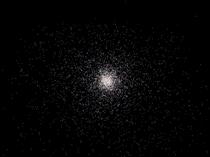
Elliptical galaxies are not flat ellipses, but they are three-dimensionally elliptical (water-melon like). Orbits of stars do not show a systematic rotation in such galaxies and are largely chaotic. Elliptical galaxies are smooth, featureless, almost spherical. Elliptical galaxies are slowly rotating objects (Bertola and Capaccioli, 1975) supported by pressure, i.e. their dynamics is dominated by the irregular motion of stars (elliptical galaxies are kinematically hot).
Some of the elliptical galaxies are thought to be very old, because they contain red giant stars that are known to be old and very little or no gas and dust. The lack of blue young stars shows that the elliptical galaxies do not form stars currently. These elliptical galaxies reached their shape after the collapse of initial protogalaxy cloud. Some ellipticals might be newer and result from a more recent evolution (see Chapter 6).
Elliptical galaxies are both the most massive galaxies containing up to a few trillion of stars (central dominant or cD galaxies at the centers of galaxy clusters) and the least massive galaxies with a few million of stars.
Hubble space telescope (HST) imaging of massive
elliptical galaxies revealed super-massive black holes in their centers. Giant
elliptical galaxy M87, for example, contains central supermassive black hole of
2 to 3 billion solar masses (![]() ).
).
Black holes
Black hole is an extremely dense object, where
the gravitational field is so powerful that nothing can escape. We can categorize
black holes through their mass as stellar black holes (BHs) with masses ![]() , intermediate black holes
(IMBHs) with masses
, intermediate black holes
(IMBHs) with masses ![]() , and supermassive
black holes (SMBHs) with masses
, and supermassive
black holes (SMBHs) with masses ![]() (Miller,
2006).
(Miller,
2006).
Disk
A thin disk consists of relatively young stars, open clusters (loose clusters of stars), middle age stars like the Sun, gas and dust (interstellar matter or ISM). Observations of disk galaxies are showing that these galaxies have the very thin disk whose radius is of order 10 kiloparsecs and thickness is of order 100 parsecs.
The most of the stars in a disk galaxy travel on
nearly circular orbits. Disk galaxies are rotationally supported, i.e. the
regular circular motion of stars (disk galaxies are kinematically cool)
dominates them. Stars in disk galaxies usually rotate with a constant velocity in
the range of ![]() to
to ![]() with only a low dispersion
of the velocity of order
with only a low dispersion
of the velocity of order ![]() .
Therefore, the angular momentum must govern the structure of disk galaxies. The
rotation of the disk prevents its gravitational collapse in a radial direction.
We all live in the Milky Way galaxy, where stars usually rotate with a velocity
of
.
Therefore, the angular momentum must govern the structure of disk galaxies. The
rotation of the disk prevents its gravitational collapse in a radial direction.
We all live in the Milky Way galaxy, where stars usually rotate with a velocity
of ![]() and with a low velocity dispersion
of about
and with a low velocity dispersion
of about ![]() .
.
It is estimated that there are approximately ![]() stars in the disk of the Milky
Way galaxy in total, most of these stars have a slightly lesser mass than the
Sun have. The Sun lies approximately 8.5 kiloparsecs from the center of the
Milky Way. Disk galaxies contain mainly blue stars that are very massive and
are known to live shortly. Because these young stars still exist in disk
galaxies, these galaxies are referred to as young galaxies. These stars are
born mainly in spiral arms. The spiral arms look like that they contain a more
mass than their surroundings. However, there is at most 5 percent more of the mass
in the spiral arms than outside of them. The formation of young massive bright
blue and ultraviolet stars makes the spiral arms look so bright. The gas is
compressed in the location of spiral arms and therefore the star formation
takes a place mainly in arms. Mature disk galaxies now contain of order
stars in the disk of the Milky
Way galaxy in total, most of these stars have a slightly lesser mass than the
Sun have. The Sun lies approximately 8.5 kiloparsecs from the center of the
Milky Way. Disk galaxies contain mainly blue stars that are very massive and
are known to live shortly. Because these young stars still exist in disk
galaxies, these galaxies are referred to as young galaxies. These stars are
born mainly in spiral arms. The spiral arms look like that they contain a more
mass than their surroundings. However, there is at most 5 percent more of the mass
in the spiral arms than outside of them. The formation of young massive bright
blue and ultraviolet stars makes the spiral arms look so bright. The gas is
compressed in the location of spiral arms and therefore the star formation
takes a place mainly in arms. Mature disk galaxies now contain of order ![]() solar masses of gas (
solar masses of gas (![]() ).
).
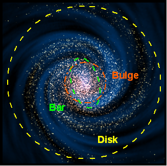
Figure 5–1: A face-on view of a disk galaxy with spiral arms, bar and bulge.
Bulge
A central bulge is a small spherical component dominated by old red stars. This galactic component of a disk galaxy resembles a miniature elliptical galaxy. The bulge surrounds the central super massive black hole. The Milky Way galaxy harbors the black hole with the mass of about 3.6 million solar masses (Eisenhauer et al., 2005). Supermassive black holes lurk at the centers of most, if not all, galaxies (Silk and Rees, 1998).
Bar
Bars are a common feature among disk galaxies. These bars have various morphologies in the sense of length, thickness, and shape. From surveys of spiral galaxies is estimated that about 75 percents of spiral galaxies have bars or ovals (Grosbøl et al., 2002). The Milky Way galaxy also has a bar (Binney, 1995).
Stellar halo
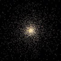
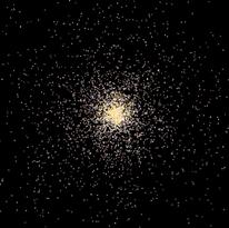
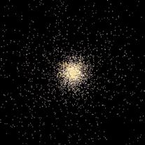
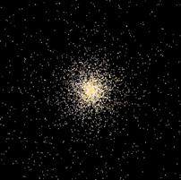
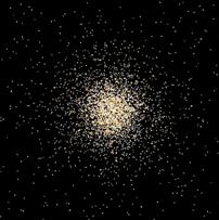
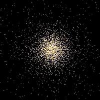
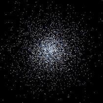
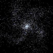
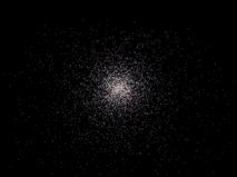
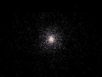
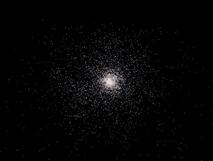
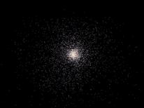
A roughly spherical halo of galaxy contains globular clusters (GCs), i.e. isolated dense stellar clusters of millions of stars, and other ISM. Like in elliptical galaxies, the motion of stars in globular clusters is chaotic. Globular clusters usually contain old red (giant) stars and are therefore very old. The stellar halo has a mass in the range of 15 to 30 percent of the mass of disk. The diameter of the halo is approximately the same as the diameter of the disk.
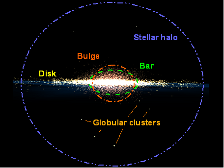
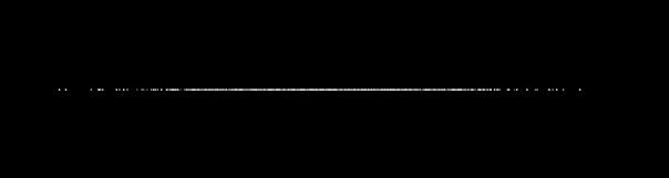
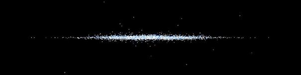
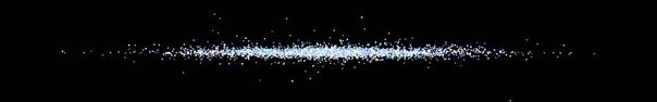
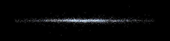
Figure 5–2: The disk galaxy as on Figure 5–1, but seen edge-on.
Galaxies did not appeared suddenly out of nothing as we will show in Chapter 6. However, it is necessary for the sake of clarity to make some simplifying hypotheses. In this chapter, we will study the evolution of galaxies by performing simulations of isolated systems that are in the steady state (equilibrium[42]).
Elliptical galaxies contain mainly stars and very little gas. They can be readily approximated with mass bodies representing stars. Disk galaxies contain larger quantities of gas, but still there is a significantly larger proportion of stars than of the gas. Galaxy is in the first approximation a large collection of stars or with even greater idealization, the ensemble of mass bodies hold together by the gravity. We can suppose that many of the properties we study in galaxy dynamics can be understood using a very simple approximation composed of following models.
Mathematical review
First, I will review some useful mathematical notions used throughout the text.
Vector quantities like ![]() are usually expressed as
are usually expressed as ![]() , where
, where ![]() are positions (components of
a vector) along unit base vectors (directions)
are positions (components of
a vector) along unit base vectors (directions) ![]() .
.
The summation convention is used during repetitive additions. For example, the equation
|
|
(5.1) |
can be rewritten as
|
|
(5.2) |
We will encounter Hamilton’s operator ![]() (pronounced “nabla” or “del”). It is defined as
(pronounced “nabla” or “del”). It is defined as
|
|
(5.3) |
We will also encounter Laplace’s operator ![]() . It is defined as
. It is defined as
|
|
(5.4) |
5.3 Gravity
In secondary school physics we are taught that the gravity is a force acting remotely and instantaneously between all bodies as was stated by Sir Isaac Newton[43], based on his observations of nature and reasoning. According to Newton’s theory “every particle of matter in the universe attracts every other particle with a force which is directly proportional to the product of their masses and inversely proportional to the square of their distances apart”.
In the mathematical description of gravity, we
will start with a scalar gravitational potential field rather than a vector
force field. Suppose we have some arrangement of mass points fixed in space and
we are interested in their cumulative effect on some given point in space. Total
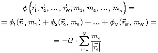
gravitational potential of N bodies with masses ![]() in a certain point in space
is additive and is given by the total sum of all potentials from individual
bodies
in a certain point in space
is additive and is given by the total sum of all potentials from individual
bodies ![]() at distances
at distances ![]() from the given point in
space as
from the given point in
space as
|
|
(5.5) |
The configuration of N point masses (the N-body
system) can be generalized to a continuous mass density distribution function ![]() , which is a function of
position
, which is a function of
position ![]() . If we write
. If we write ![]() as a function of coordinates
as a function of coordinates
![]() then
then ![]() is the mass contained in a
little box of volume
is the mass contained in a
little box of volume ![]() , located at the
point
, located at the
point ![]() . A mass density
. A mass density ![]() in a specific place is given
by the sum of mass sources (point masses) in an infinitely small volume
element. The mass density distribution function
in a specific place is given
by the sum of mass sources (point masses) in an infinitely small volume
element. The mass density distribution function ![]() is
the function describing the distribution of matter (stars) in the system (galaxy).
A transition from a discrete to continuous form can be approximately expressed
as
is
the function describing the distribution of matter (stars) in the system (galaxy).
A transition from a discrete to continuous form can be approximately expressed
as ![]() .
.
In a similar way, the gravitational potential generated by the continuous mass distribution instead of individual bodies as sources of the potential can be expressed continuously. Summation (5.5) is turning into integration in places (macroscopically) continuously filled with matter.
The gradient of the potential is then the
gravitational force acting on a body with a unit mass, apart from a minus sign.
The exploring body of the unit mass will experience at any point given by a position
![]() force
force
|
|
(5.6) |
This quantity ![]() is
called the intensity of gravitational field.
is
called the intensity of gravitational field.
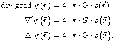
With continuous functions, we may use Poisson’s equation (Greiner, 2004)
|
|
(5.7) |
Here we get a connection between the gravitational
potential ![]() and the mass density
and the mass density ![]() . Poisson’s equation serves
as one of the principal governing equations in our examination of stability,
structure and dynamics of self-gravitating systems. The mass density required
for the generation of the potential can be found by solving Poisson’s equation.
On the other side, from the known mass density, we can determine the
gravitational potential through Poisson’s equation.
. Poisson’s equation serves
as one of the principal governing equations in our examination of stability,
structure and dynamics of self-gravitating systems. The mass density required
for the generation of the potential can be found by solving Poisson’s equation.
On the other side, from the known mass density, we can determine the
gravitational potential through Poisson’s equation.
Different components of galaxies (disk, bulge… and halo) have their own mass density function within the global gravitational potential. Poisson’s equation gives us a relation between them. For a self-gravity model, we must find the global gravitational potential, in which the mass density of all parts of a galaxy is combined as
|
|
(5.8) |
5.4 Initial conditions for spherical systems
As was described in Chapter 4.1, initial conditions for the N-body
system must be set up. The most convenient is to start with elliptical
galaxies. Systems with a spherical symmetry can be described by functions
depending only on a one-dimensional distance ![]() from
the center of the system. In the centrally symmetric mass distribution with the
spherical symmetry are the mass density
from
the center of the system. In the centrally symmetric mass distribution with the
spherical symmetry are the mass density ![]() and
gravitational potential
and
gravitational potential ![]() same in
each direction with the origin at the center of the system. The spherical
symmetry therefore implies
same in
each direction with the origin at the center of the system. The spherical
symmetry therefore implies ![]() and
and ![]() . Poisson’s equation in one dimension
is expressed as
. Poisson’s equation in one dimension
is expressed as
|
|
(5.9) |
A uniform sphere is one of the simplest approximations of the spherical system with the uniform density distribution function (volume density) given by
|
|
(5.10) |
where ![]() is the
mass of the sphere and
is the
mass of the sphere and ![]() is its radius. As
we would expect from the mass density distribution function
is its radius. As
we would expect from the mass density distribution function ![]() , outside the sphere
potential falls off as in Keplerian case. This is known as Newton’s theorem. It
states that “a body inside a spherical shell of matter experiences no net
gravitational force from the shell” (the mass exterior to the shell has no
effect) and that “the gravitational force on a body lying outside a closed
spherical shell experiences a gravitational force which is the same as if all
the matter in the shell was concentrated at a point at its center” (Greiner,
2004).
, outside the sphere
potential falls off as in Keplerian case. This is known as Newton’s theorem. It
states that “a body inside a spherical shell of matter experiences no net
gravitational force from the shell” (the mass exterior to the shell has no
effect) and that “the gravitational force on a body lying outside a closed
spherical shell experiences a gravitational force which is the same as if all
the matter in the shell was concentrated at a point at its center” (Greiner,
2004).
Isothermal sphere has interesting property since its rotational velocity is unchanging with radius (it is constant). Therefore the isothermal sphere is useful for modeling flat rotational curves (more on Chapter 5.11). The mass density distribution function of isothermal sphere is given by
|
|
(5.11) |
where ![]() is a central
density and a is a scale length. This distribution function (see
is a central
density and a is a scale length. This distribution function (see
Figure 5–3) gives the system with an infinite mass and must be therefore
truncated at some distance from the center. Cut-off radius must be imposed for
a finite total mass.
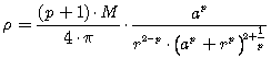
We should now turn to more realistic density distribution functions that mimic spherical components of galaxy. Plummer’s (1911) model is such a simple approximation with the mass density distribution function given by
|
|
(5.12) |
Another more realistic model is Hernquist’s (1990) model given by
|
|
(5.13) |
Plummer’s and Hernquist’s models are members of the same family of models (Evans and An, 2005). They can be both described by the mass density distribution function as
|
|
(5.14) |
where parameter p is a positive number.
The case ![]() is Hernquist’s model and the
case
is Hernquist’s model and the
case ![]() Plummer’s model.
Plummer’s model.
Another realistic model is Jaffe’s (1983) model expressed as
|
|
(5.15) |
5.5 Units and scales
It is often useful to reduce units and equations
describing a physical system to a dimensionless form, both for physical insight
and numerical convenience. Let us imagine that we are using the gravitational
constant in SI units that is of order ![]() .
However, typical distances in the world of galaxies are of order
.
However, typical distances in the world of galaxies are of order ![]() in SI units. A finite numerical
representation of real numbers in a digital computer will most likely yield to
large numerical round-off errors when we will compute with numbers of tens
orders different. Therefore, we will use non-dimensional units throughout our
simulations. We adopt
in SI units. A finite numerical
representation of real numbers in a digital computer will most likely yield to
large numerical round-off errors when we will compute with numbers of tens
orders different. Therefore, we will use non-dimensional units throughout our
simulations. We adopt ![]() for Newton’s gravity constant, a total mass of system
for Newton’s gravity constant, a total mass of system ![]() and
a scale length
and
a scale length ![]() is also set equal
to 1. As a general rule, all quantities in this text are given in these intrinsically
scale free units unless otherwise noted.
is also set equal
to 1. As a general rule, all quantities in this text are given in these intrinsically
scale free units unless otherwise noted.
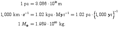
It is useful to summarize some commonly used units:
|
|
|
Let us consider a practical choice of units on
measures of galaxies. A typical disk galaxy has a size of orders of
kiloparsecs, contains hundreds of billions of stars, and a rotational velocity
in such galaxy is usually up to ![]() . The
models may be therefore compared with real galaxies using, for example, the
following scaling
. The
models may be therefore compared with real galaxies using, for example, the
following scaling
|
|
|
where we employed a convention to write ![]() for the unit of quantity
for the unit of quantity ![]() .
. ![]() is
a unit length,
is
a unit length, ![]() is a unit mass,
and
is a unit mass,
and ![]() is a unit velocity. With
these, the unit time can be derived as
is a unit velocity. With
these, the unit time can be derived as
|
|
(5.16) |
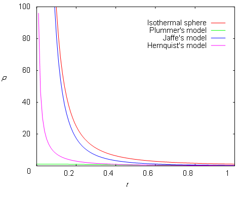
Figure 5–3: Density profiles of spherical components for modeling galaxies. All
have ![]() .
.
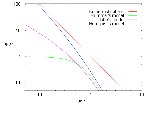
Figure 5–4: Density profiles of spherical components for modeling galaxies on
logarithmical scale axes. All have ![]() .
.
5.6 Positions of bodies in galaxy
A probability ![]() that
we will find a body (i.e. star) in the volume of spherical shell limited by
radii
that
we will find a body (i.e. star) in the volume of spherical shell limited by
radii ![]() relates to the radial mass
density distribution function
relates to the radial mass
density distribution function ![]() as
as
|
|
(5.17) |
First, we will introduce the amount of mass in the
spherical system bounded by the sphere with a radius ![]() . This quantity is called a cumulative
mass distribution
. This quantity is called a cumulative
mass distribution ![]() and is given by
and is given by
|
|
(5.18) |
In numerical formulation is the density profile ![]() numerically integrated with the
radius
numerically integrated with the
radius ![]() changing between a minimal
radius equal to zero and a maximum radius
changing between a minimal
radius equal to zero and a maximum radius ![]() .
The cumulative mass distribution
.
The cumulative mass distribution ![]() of a
model is tabulated on a grid with points spaced logarithmically in
of a
model is tabulated on a grid with points spaced logarithmically in ![]() .
To check and compare
numerical results with analytic solutions, we have plotted the analytic and
numeric
.
To check and compare
numerical results with analytic solutions, we have plotted the analytic and
numeric ![]() of Plummer’s model to see
the difference (Figure 5–5).
of Plummer’s model to see
the difference (Figure 5–5).
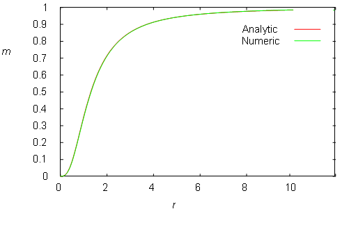
Figure 5–5: The cumulative mass of Plummer’s model computed in an analytic and numeric form. The numeric representation is so precise that no deviation from the analytic expression can be seen. The numeric representation (green curve) completely covers analytic representation (red curve).
The cumulative mass distribution ![]() is essentially a probability
distribution function (PDF). Numerical libraries contain a variety of random
number generators, but how can we realize an arbitrary PDF?
is essentially a probability
distribution function (PDF). Numerical libraries contain a variety of random
number generators, but how can we realize an arbitrary PDF?
Given the known PDF, it can be realized by a random
(Monte Carlo[44])
sampling from the PDF. We can find the maximum ![]() of
the function
of
the function ![]() (overall mass of the system
of bodies); we also know the maximum radius
(overall mass of the system
of bodies); we also know the maximum radius ![]() .
Then, we generate a couple of random numbers with a uniform distribution. We generate a random number R with the
uniform distribution in an interval
.
Then, we generate a couple of random numbers with a uniform distribution. We generate a random number R with the
uniform distribution in an interval ![]() and
expand it (multiply by
and
expand it (multiply by ![]() ) to
) to ![]() range. Then we generate a second
random number P with the uniform distribution in interval
range. Then we generate a second
random number P with the uniform distribution in interval ![]() and expand it (multiply by
and expand it (multiply by ![]() ) to
) to ![]() range. If the value of
function
range. If the value of
function ![]() is equal or smaller than the
random number P (so that the number P is under the graph of point
is equal or smaller than the
random number P (so that the number P is under the graph of point
![]() ) then we will accept the
distance R. Otherwise, we reject this number, generate again two new
random numbers R and P and perform the test again. The method is
called acceptance-rejection method. It was used by John von Neumann[45] and
is therefore sometimes called “von Neumann’s method”.
) then we will accept the
distance R. Otherwise, we reject this number, generate again two new
random numbers R and P and perform the test again. The method is
called acceptance-rejection method. It was used by John von Neumann[45] and
is therefore sometimes called “von Neumann’s method”.
We may discover also other method for sampling
from the arbitrary PDF.
We may invert the function ![]() to
a function
to
a function ![]() and thus obtain
and thus obtain ![]() . We can find the maximum
value
. We can find the maximum
value ![]() of the function
of the function ![]() for
for ![]() . Then we generate the random
number M from the uniform distribution and expand it to interval
. Then we generate the random
number M from the uniform distribution and expand it to interval ![]() . Finally, we will receive the
position of the body by evaluating
. Finally, we will receive the
position of the body by evaluating ![]() .
.
Up to now, all functions were one-dimensional.
Now, we must scatter bodies to all three dimensions. The initial radius ![]() of a body is randomly
determined according to the radial surface density distribution function
of a body is randomly
determined according to the radial surface density distribution function ![]() . The initial angles
. The initial angles ![]() and
and ![]() are drawn uniformly between
are drawn uniformly between ![]() and
and ![]() . Particles are then positioned
in three dimensions using
. Particles are then positioned
in three dimensions using
|
|
(5.19) |
To have a body on a stable orbit, its kinetic
energy ![]() must be exactly the same as a
potential energy
must be exactly the same as a
potential energy ![]() , i.e.,
, i.e., ![]() or
or ![]() [46]. The
kinetic energy is defined as
[46]. The
kinetic energy is defined as ![]() , where m,
v are the mass and velocity of the body, respectively. The potential energy
is defined as
, where m,
v are the mass and velocity of the body, respectively. The potential energy
is defined as ![]() , where
, where ![]() is the distance of the body
from the center of the system. The potential energy characterizes a mutual
force between bodies – the potential energy is shared at least between
two bodies. The gravitational potential
is the distance of the body
from the center of the system. The potential energy characterizes a mutual
force between bodies – the potential energy is shared at least between
two bodies. The gravitational potential ![]() is
always negative. The potential energy
is
always negative. The potential energy ![]() is
resulting from the interaction of the body and the companion system.
is
resulting from the interaction of the body and the companion system.
The velocity for the stable orbit can be derived as
|
|
(5.20) |
The body will stay in the system until its
kinetic energy ![]() will not be
greater than the potential energy
will not be
greater than the potential energy ![]() of
gravity that binds this body to the system. When
of
gravity that binds this body to the system. When ![]() ,
the body will leave the system with so called escape velocity
,
the body will leave the system with so called escape velocity ![]() . This velocity can be easily
derived for the spherically symmetric system, when we take into account Newton’s theorems. Then the whole system is looking like the mass point of a mass M
with the gravitational potential
. This velocity can be easily
derived for the spherically symmetric system, when we take into account Newton’s theorems. Then the whole system is looking like the mass point of a mass M
with the gravitational potential ![]() and the
escape velocity required for the body to escape infinitely far from the gravitational
field will be
and the
escape velocity required for the body to escape infinitely far from the gravitational
field will be
|
|
(5.21) |
The body will stay in the system for ![]() .
.
Phase-space distribution function
An equilibrium spherical system depends on the
phase-space coordinates ![]() (Lynden-Bell,
1962). The structure of a galaxy is defined by a distribution function
(Lynden-Bell,
1962). The structure of a galaxy is defined by a distribution function ![]() in the imaginary space
called phase-space with 6 dimensions (three spatial coordinates for positions
and three corresponding velocity components) at each moment (time) t. The
phase-space is given by the product of configuration space (positional space,
represents generalized coordinates) and velocity space (represents generalized
momentum).
in the imaginary space
called phase-space with 6 dimensions (three spatial coordinates for positions
and three corresponding velocity components) at each moment (time) t. The
phase-space is given by the product of configuration space (positional space,
represents generalized coordinates) and velocity space (represents generalized
momentum).
Such a system of bodies is subjected to the potential
![]() that is completely described
by its phase-space distribution function
that is completely described
by its phase-space distribution function ![]() .
It is a probability density of finding some mean number
.
It is a probability density of finding some mean number ![]() of stars
of stars ![]() in a small box
in a small box ![]() near a position
near a position ![]() , i.e. between
, i.e. between ![]() and
and ![]() ,
, ![]() and
and
![]() ,
, ![]() and
and
![]() , and velocities in the range
, and velocities in the range
![]() about
about ![]() , i.e. between
, i.e. between ![]() and
and ![]() ,
, ![]() and
and
![]() ,
, ![]() and
and
![]() . The probability density is
never negative.
. The probability density is
never negative.
We have already found the position of the star
in the system (a 3D position in the configuration sub-space of 6D phase-space)
as was described in Chapter 5.6.
Now, we must find the range of velocities ![]() in
the phase-space for the concrete position and also a correct statistical weight
that tells us what probability distribution function is for
in
the phase-space for the concrete position and also a correct statistical weight
that tells us what probability distribution function is for ![]() . As was shown in Equation (5.21), the escape velocity is given by the gravitational
potential energy that comes from the gravitational potential of the system at the
given point of space. The velocity distribution function at the position of
each particle can be found from the distribution function
. As was shown in Equation (5.21), the escape velocity is given by the gravitational
potential energy that comes from the gravitational potential of the system at the
given point of space. The velocity distribution function at the position of
each particle can be found from the distribution function ![]() . The distribution function f
is assumed to be zero
. The distribution function f
is assumed to be zero ![]() for energies
for energies ![]() greater than zero (while
assuming a unit mass), because the stars with the positive energy will leave
the system.
greater than zero (while
assuming a unit mass), because the stars with the positive energy will leave
the system.
We must find the concrete phase-space
distribution function ![]() for the desired
models. The probability isotropic distribution function f of any
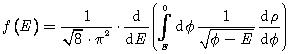
spherical model depends only on the overall specific energy E (energy
per unit mass) of the system of stars and is available as (Eddington, 1916)[47]
for the desired
models. The probability isotropic distribution function f of any
spherical model depends only on the overall specific energy E (energy
per unit mass) of the system of stars and is available as (Eddington, 1916)[47]
|
|
(5.22) |
Abel integral transform is required to relate
density profile ![]() of models and the distribution
function
of models and the distribution
function ![]() to the potential generated
by
to the potential generated
by ![]() . However, analytical
distribution functions are known for only a handful of models, such as e.g.
Plummer’s model. In order to generate any model that is more realistic, one has
to find the steady state distribution function
. However, analytical
distribution functions are known for only a handful of models, such as e.g.
Plummer’s model. In order to generate any model that is more realistic, one has
to find the steady state distribution function ![]() that
reproduces the desired density
that
reproduces the desired density ![]() numerically.
numerically.
Gravitational potential
In order to solve Equation (5.22), we must find the gravitational
potential ![]() connected to the mass
density
connected to the mass
density ![]() (that we have for various
spherical models) through Poisson’s equation (5.7). Let us remind Poisson’s equation in
one dimension given by
(that we have for various
spherical models) through Poisson’s equation (5.7). Let us remind Poisson’s equation in
one dimension given by
|
|
(5.23) |
The cumulative
mass distribution ![]() relates to the gravitational
potential
relates to the gravitational
potential ![]() through Poisson’s equation
as follows
through Poisson’s equation
as follows
|
|
(5.24) |
In the numerical formulation is the gravitational
potential ![]() determined by numerical
integration of the cumulative mass distribution
determined by numerical
integration of the cumulative mass distribution ![]() and
is tabulated on a grid between the minimal radius equal to zero and radius
equal to ten times the maximum radius
and
is tabulated on a grid between the minimal radius equal to zero and radius
equal to ten times the maximum radius ![]() with
grid points spaced logarithmically in
with
grid points spaced logarithmically in ![]() .
The cumulative mass distribution
.
The cumulative mass distribution ![]() is
obtained by the interpolation of the grid points.
is
obtained by the interpolation of the grid points.
Determination of distribution function
The integrand in
Equation (5.22) depends on the derivative of the
density ![]() . We must therefore express
mass density
. We must therefore express
mass density ![]() as the function of the gravitational
potential
as the function of the gravitational
potential ![]() . Both the mass density
. Both the mass density ![]() and the gravitational
potential
and the gravitational
potential ![]() are obtained from a numerical
interpolation of
are obtained from a numerical
interpolation of ![]() and
and ![]() at the logarithmically
spaced points
at the logarithmically
spaced points ![]() and acquired
values are placed on a grid that represents
and acquired
values are placed on a grid that represents ![]() .
The numerical derivation is then performed on the function
.
The numerical derivation is then performed on the function ![]() . Numerical integration is
applied to the integral from Equation (5.22) and the result is placed on the grid
of
. Numerical integration is
applied to the integral from Equation (5.22) and the result is placed on the grid
of ![]() evaluated at logarithmically
spaced points
evaluated at logarithmically
spaced points ![]() . Finally, Equation
(5.22) must be differentiated;
and we get the distribution function
. Finally, Equation
(5.22) must be differentiated;
and we get the distribution function ![]() .
.
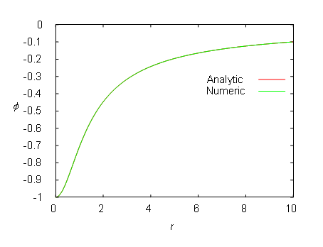
Figure 5–6: The gravitational potential of Plummer’s model computed in an analytic and numeric form. The numeric representation is so precise that no deviation from the analytic form can be seen.
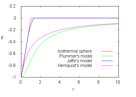
Figure 5–7: Numerically computed gravitational potentials of various spherical models.
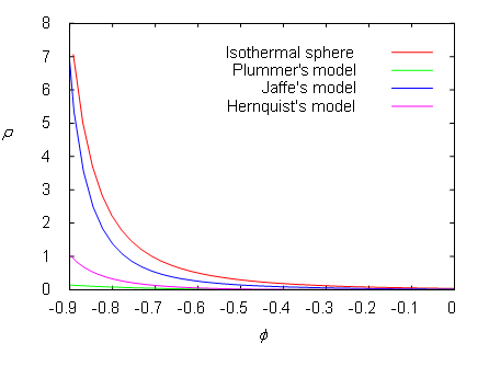
Figure 5–8: The mass density distribution ![]() as the function of the gravitational potential
as the function of the gravitational potential ![]() .
.
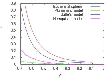
Figure 5–9: Numerically computed distribution function of various spherical models.
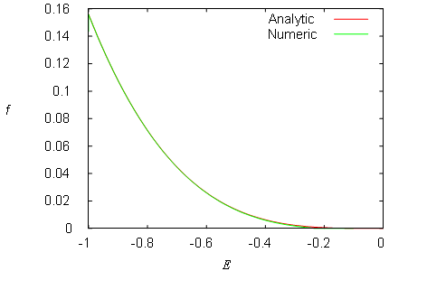
Figure 5–10: The distribution function ![]() of the Plummer’s model computed in the analytic and
numeric form. A minute deviation can be seen as the function is approaching
zero.
of the Plummer’s model computed in the analytic and
numeric form. A minute deviation can be seen as the function is approaching
zero.
Once the N-body system is generated, its
realization must be verified. Every closed system held together by the gravity must
globally obey the virial theorem[48].
The virial theorem states that the mean values of the kinetic energy ![]() and potential energy
and potential energy ![]() are related as
are related as ![]() or
or ![]() in the closed system. The
total energy
in the closed system. The
total energy ![]() is conserved.
is conserved.
Given a total mass M and the mean kinetic
energy ![]() of the system of stars, we
may get from the definition of the kinetic energy a characteristic velocity
of the system of stars, we
may get from the definition of the kinetic energy a characteristic velocity
|
|
(5.25) |
We can also define a characteristic length (Meylan and Heggie, 1996)
|
|
(5.26) |
These characteristic quantities are sometimes known as the virial velocity and radius. Their ratio is an estimate of time that a typical star takes to cross the system. The crossing time is a measure of the time that take for a star to traverse the diameter of the system. The crossing time is defined (Meylan and Heggie, 1996) as
|
|
(5.27) |
where ![]() is a
measure of the size of the system and
is a
measure of the size of the system and ![]() a
measure of the mean stellar velocity. We choose
a
measure of the mean stellar velocity. We choose ![]() and
and
![]() to be equal to
to be equal to ![]() and
and ![]() , respectively.
, respectively.
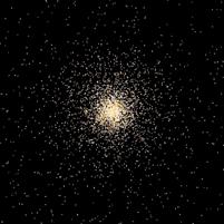
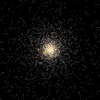
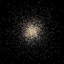
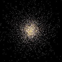
Our first objective is a simulation of elliptical galaxies with an eccentricity of zero (spherical galaxies). We will perform the simulation of two spherical systems – Plummer’s and Hernquist’s models.
We will use a program for initial conditions
generation to create a spherical galaxy consisting of stars with a position,
velocity and mass each. We will evolve initial conditions with the Barnes-Hut N-body
simulation code with the opening angle ![]() .
.
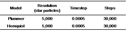
Table 5–1: Parameters of simulation for Plummer’s and Hernquist’s model.
Model realization is in the dimensionless system
of units. Gravitational forces were calculated after
smoothing the mass distribution using the softening length ![]() . Model is comparable to a real-world
dwarf spherical galaxy with following radius, mass and Newton’s gravitation
constant
. Model is comparable to a real-world
dwarf spherical galaxy with following radius, mass and Newton’s gravitation
constant
|
|
|
The time unit is comparable to ![]() , the timestep to
, the timestep to ![]() and the overall simulation
with
and the overall simulation
with ![]() steps covers
steps covers ![]() .
.
|
|
|
|
|
Start |
224 million years |
448 million years |
|
|
|
|
|
|
|
|
|
671 million years |
895 million years |
1.12 billion years |
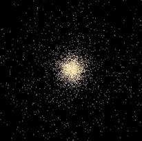
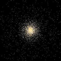
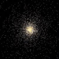
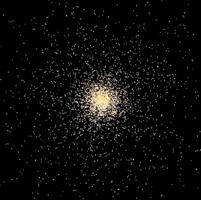
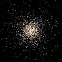
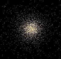
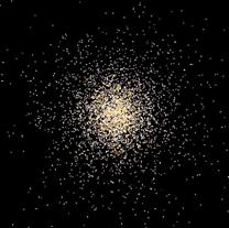
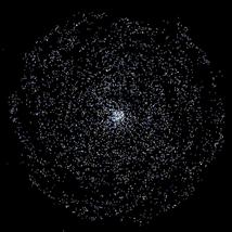
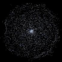
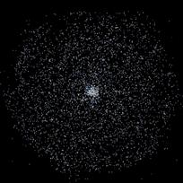
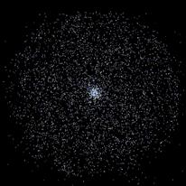
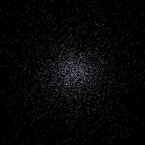
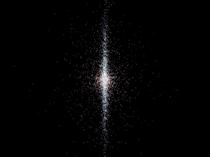
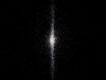
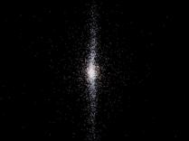
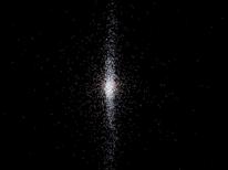
Figure 5–11: A time sequence of Hernquist’s model in the xy plane. Practically no evolution can be seen.
|
|
|
|
|
Start |
224 million years |
448 million years |
|
|
|
|
|
|
|
|
|
671 million years |
895 million years |
1.12 billion years |
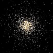
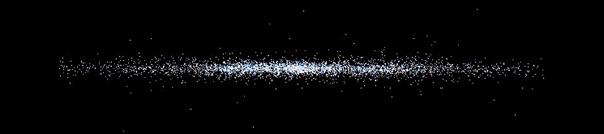
Figure 5–12: A time sequence of Hernquist’s model in the yz plane.
|
|
|
|
|
Start |
224 million years |
448 million years |
|
|
|
|
|
|
|
|
|
671 million years |
895 million years |
1.12 billion years |
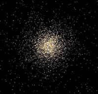
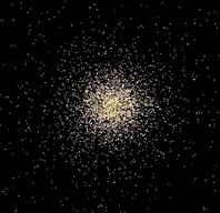
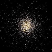
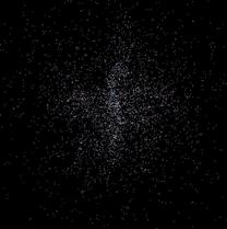
Figure 5–13: A time sequence of Plummer’s model in the xy plane. Practically no evolution can be seen.
|
|
|
|
|
Start |
224 million years |
448 million years |
|
|
|
|
|
|
|
|
|
671 million years |
895 million years |
1.12 billion years |
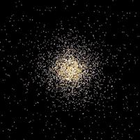
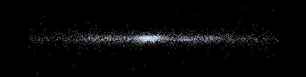
Figure 5–14: A time sequence of Plummer’s model in the yz plane.
Stability test of the initial models shows a little evolution in these models. Both Hernquist’s and Plummer’s models are in the dynamic equilibrium from the beginning.
5.9 Initial conditions for flattened systems
A spiral galaxy is flat and can be represented by a flattened potential. The disk of the spiral galaxy is generally very flat and we will describe them as infinitely thin. We will suppose that disks are axisymmetrical and therefore, initial conditions will be set up in cylindrical coordinates.
An initial angle ![]() is
drawn uniformly between
is
drawn uniformly between ![]() and
and ![]() . In the xy plane are disk
particles positioned using
. In the xy plane are disk
particles positioned using
|
|
(5.28) |
Stars in the disk have only circular velocities (so called cold disk, where no random motions are induced). Disk rotation is generated to be counter-clockwise in the xy plane (right handed Cartesian coordinate system is completed with z-axis and disk rotation is chosen to by given by the right hand rule with a thumb along z-axis).
A reasonable approximation for the disk galaxy
is Kuzmin’s disk. Kuzmin found in 1956 the potential of an infinitesimally
razor-thin disk with Plummer’s potential in the plane of the disk. The initial
mass density distribution (surface density) ![]() of
Kuzmin’s disk in the disk plane is
of
Kuzmin’s disk in the disk plane is
|
|
(5.29) |
where ![]() is a distance
from the center of the disk and
is a distance
from the center of the disk and ![]() is a radial
scale length. This mass density belongs to a more general family of disks
introduced by Toomre (1963).
is a radial
scale length. This mass density belongs to a more general family of disks
introduced by Toomre (1963).
Bodies in an exponential disk are distributed in the plane with the surface mass density distribution given by
|
|
(5.30) |
Kepler’s disk has the potential of a
point mass ![]() given by
given by ![]() . Its rotation is that obeyed
by the planets in the solar system and Kepler’s three laws. A circular velocity
computed after introducing Kepler’s potential is
. Its rotation is that obeyed
by the planets in the solar system and Kepler’s three laws. A circular velocity
computed after introducing Kepler’s potential is
|
|
(5.31) |
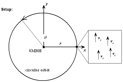
Figure 5–15: An initial setup of Kepler’s disk with circular velocities.
5.10 Disk galaxies
Kepler’s model
As the first approximation, we can model a disk galaxy with Kepler’s model. As the planets in the solar system revolve around the Sun, also the stars (with planetary systems) in the disk galaxy are revolving on (nearly) circular orbits around the supermassive black hole at the center. The two massive bodies (SMBH and single star) are essentially unaffected by the third body (other stars).
Let us assume that the galaxy is made of two components: the stellar disk with uniformly distributed stars and the super-massive black hole. A model realization is in the dimensionless system of units. We will evolve initial conditions with the Barnes-Hut N-body simulation code.
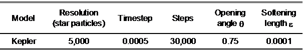
Table 5–2: Parameters of the Kepler’s disk simulation.
The conversion to physical units is performed by scaling the Kepler’s digital galaxy to the system with known physical properties. If we scale it to the disk of the Milky Way galaxy, the unit length, unit mass, unit velocity, gravitational constant and unit time are
|
|
|
The timestep is therefore equal to ![]() and the overall simulation
covers
and the overall simulation
covers ![]() .
.
|
|
|
|
|
Start |
205 million years |
409 million years |
|
|
|
|
|
|
|
|
|
|
|
|
|
614 million years |
818 million years |
1.02 billion years |
Figure 5–16: A time sequence for Kepler’s disk model in the xy plane. The disk is ideally flat in the yz plane.
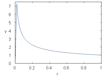
Figure 5–17: A rotation curve[49] of Kepler’s model.
5.11 Rotation curves
We will now compare a rotation curve from the simulations of Kepler’s disk with a rotation curve of a real galaxy as measured by a real experiment. Such work can be carried out with a radio telescope that traces neutral hydrogen (HI) atoms and carbon monoxide (CO) molecules. HI atoms are hard to observe, but CO molecules are copying the presence of HI atoms and their motion. Spectroscopy and the Doppler Effect permits us to measure the speed of gas orbiting around the center of the galaxy.
These observations of galactic rotation curves in disk galaxies have revealed that rather than falling-off as we can see in the plot of our computer simulation of Kepler’s disk (see Figure 5–17) and that is in an agreement with Newtonian physics and observed mass, the rotational velocities remain constant at large radii. This is valid for rotation curves of the Milky Way galaxy and other real galaxies (Fuchs et al., 1998).
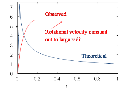
Figure 5–18: Rotation curves: Theoretical (based on Newton’s law of gravity and visible matter) and experimental (based on observations).
Based on an astronomical observation of a mass distribution in disk galaxies can be inferred that the number of stars is dropping towards the edge of the stellar disk. From Newton’s law of gravity, we obtain
|
|
(5.32) |
where ![]() is the orbital
velocity of a star at the distance
is the orbital
velocity of a star at the distance ![]() from the
center of the galaxy. The cumulative mass inside radius
from the
center of the galaxy. The cumulative mass inside radius ![]() is
is
|
|
(5.33) |
If the orbital velocity ![]() is constant with
increasing
is constant with
increasing ![]() (as is known from
observations) then for
(as is known from
observations) then for
G = const. the only term in Equation (5.33) that can change with increasing ![]() is
is ![]() . The cumulative mass
. The cumulative mass ![]() must grow even in vast
distances from galaxy center. However, observed light or luminosity
must grow even in vast
distances from galaxy center. However, observed light or luminosity ![]() that is believed to trace the
matter distribution tends to a finite limit as we reach the edge of the
luminous material in the galaxy. Therefore, the flatness of the rotation curve
in large distances from the center of the disk, where number of stars is
beginning to drop, cannot be explained by the visible mass alone.
that is believed to trace the
matter distribution tends to a finite limit as we reach the edge of the
luminous material in the galaxy. Therefore, the flatness of the rotation curve
in large distances from the center of the disk, where number of stars is
beginning to drop, cannot be explained by the visible mass alone.
Dark matter
It is supposed that invisible matter supplies
this missing gravity. Jan H. Oort (1932) studying the motion of stars in the
Milky Way galaxy was the first one, who noticed that some matter in our galaxy
is “missing”. The flat rotation curves of spiral galaxies at large
galactocentric distance suggest that the halo of the invisible matter might
exist around spiral galaxies; this dark halo might continue to contribute to ![]() out to very large radii.
Fritz Zwicky[50]
studied the motion of galaxies within Coma cluster of galaxies in 1933. He
discovered that galaxy velocities are so large that they should fly out of the
galaxy cluster long ago. Since the cluster shows no signs of flying apart, some
force of invisible source must hold it together. It is generally supposed that some
additional matter invisible to us must gravitationally bound these galaxies
together (Zwicky, 1937).
out to very large radii.
Fritz Zwicky[50]
studied the motion of galaxies within Coma cluster of galaxies in 1933. He
discovered that galaxy velocities are so large that they should fly out of the
galaxy cluster long ago. Since the cluster shows no signs of flying apart, some
force of invisible source must hold it together. It is generally supposed that some
additional matter invisible to us must gravitationally bound these galaxies
together (Zwicky, 1937).
However, idea of dark matter (DM) was not accepted till extensive observational results of Rubin and Ford (1970). Visible parts of the spiral galaxy and the gas layers cannot account for the observed high rotation velocities in the outer parts of spirals, if the stellar mass-to-light ratio is constant with the radius. This is an indirect evidence that luminous portions of galaxies represent only a small fraction of the total galactic mass. Pioneering simulations of galaxies performed by Ostriker and Peebles (1973) also revealed that the inclusion of the massive halo will stabilize a galaxy disk against strong axisymmetric instability. Otherwise, the galaxy simply flies apart. The Milky Way and other disk galaxies may be therefore embedded in halos of unseen matter.
Orbits of stars in real disk galaxies are not
perfectly circular. We will create more realistic models of the disk galaxy
with a hot disk, where a velocity dispersion (fluctuation, deviation) is
introduced. A way to quantify velocity dispersion in the disk is the Toomre’s
(1964) parameter ![]() expressed as
expressed as
|
|
(5.34) |
where ![]() is the
radial velocity dispersion,
is the
radial velocity dispersion, ![]() is the
frequency of small oscillation about the circular radius (local Lindblad epicyclic
frequency) and
is the
frequency of small oscillation about the circular radius (local Lindblad epicyclic
frequency) and ![]() is the stellar
surface density. The stability criterion against axisymmetric perturbations
requires for the stellar disk to set
is the stellar
surface density. The stability criterion against axisymmetric perturbations
requires for the stellar disk to set ![]() . For
. For ![]() , the disk is locally
unstable and
, the disk is locally
unstable and ![]() corresponds to the cold
disk. The epicyclic frequency is opt as
corresponds to the cold
disk. The epicyclic frequency is opt as ![]() ,
where
,
where ![]() is an angular velocity
is an angular velocity ![]() .
.
Tangential (azimuthal) velocity dispersion ![]() is expressed as
is expressed as
|
|
(5.35) |
Vertical velocity dispersion (dispersion in a direction, which is perpendicular to the disk plane) is chosen as the part of tangential velocity dispersion as
|
|
(5.36) |
From Equation (5.36) can be seen that even if the initial mass density of the disk is planar, vertical dispersion will lead to the thickening of the ideally flat disk.
Hot disk realizations
We will create a disk with kinematically hot
(supported by random motions, rather than the rotational motion) stars. The
thickness of the disk is set such that Toomre’s stability criterion is
satisfied. The radial velocity dispersion ![]() corresponds
to the value of the Solar neighborhood, i.e.
corresponds
to the value of the Solar neighborhood, i.e. ![]() .
The Gaussian-distributed random velocity dispersions are equal to
.
The Gaussian-distributed random velocity dispersions are equal to ![]() ,
, ![]() and
and
![]() .
.
Kuzmin’s and exponential model
We will use a program for initial conditions
generation to create a disk galaxy. A model realization
is in the system of units in which the gravitational
constant ![]() , the total mass
, the total mass ![]() , and the scale radius
, and the scale radius ![]() , are all equal to unity. We will evolve initial conditions with the Barnes-Hut
N-body simulation code with the opening angle
, are all equal to unity. We will evolve initial conditions with the Barnes-Hut
N-body simulation code with the opening angle ![]() and the softening length
and the softening length ![]() .
.
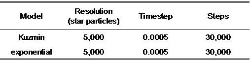
Table 5–3: Parameters of the Kuzmin’s and exponential model simulations.
The timestep was set equal to ![]() and the overall simulation
covers
and the overall simulation
covers ![]() .
.
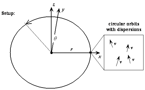
Figure 5–19: An initial setup for the hot disk with the velocity dispersion added to circular velocities.
|
|
|
|
|
Start |
205 million years |
409 million years |
|
|
|
|
|
|
|
|
|
614 million years |
818 million years |
1.02 billion years |
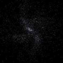
Figure 5–20: A time
sequence for the hot exponential disk with ![]() in
the xy plane evolved with the Barnes-Hut N-body algorithm.
in
the xy plane evolved with the Barnes-Hut N-body algorithm.
|
|
|
Start |
|
|
|
205 million years |
|
|
|
409 million years |
|
|
|
614 million years |
|
|
|
818 million years |
|
|
|
1.02 billion years |
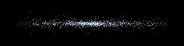
Figure 5–21: A time
sequence for the hot exponential disk with ![]() in
the yz plane evolved with the Barnes-Hut N-body algorithm. The
thickening caused by the random motion of stars can be seen.
in
the yz plane evolved with the Barnes-Hut N-body algorithm. The
thickening caused by the random motion of stars can be seen.
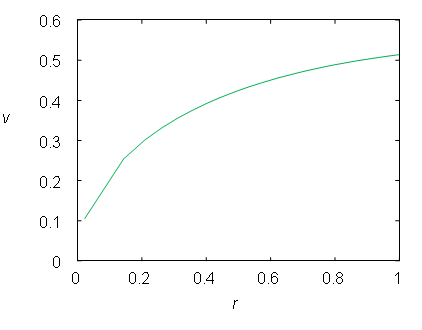
Figure 5–22: The rotation curve of the exponential disk.
|
|
|
|
|
Start |
205 million years |
409 million years |
|
|
|
|
|
|
|
|
|
614 million years |
818 million years |
1.02 billion years |
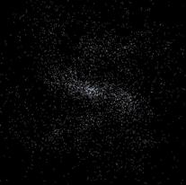
Figure 5–23: A time
sequence for the hot Kuzmin’s disk with ![]() in
the xy plane evolved with the Barnes-Hut N-body algorithm.
in
the xy plane evolved with the Barnes-Hut N-body algorithm.
|
|
|
Start |
|
|
|
205 million years |
|
|
|
409 million years |
|
|
|
614 million years |
|
|
|
818 million years |
|
|
|
1.02 billion years |
Figure 5–24: A time
sequence for the hot Kuzmin’s disk with ![]() in
the yz plane evolved with the Barnes-Hut N-body algorithm. The
thickening caused by the random motion of stars can be seen.
in
the yz plane evolved with the Barnes-Hut N-body algorithm. The
thickening caused by the random motion of stars can be seen.
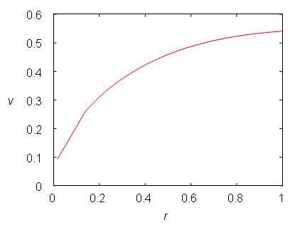
Figure 5–25: The rotation curve of Kuzmin’s disk.
First, we will check the stability of the model. The whole simulation is showing a continuous evolution and changes of both disks. After the formation of a strong axisymmetric instability, the system relaxes to a steady state. After relaxation, the system forgets its initial conditions.
Large-scale deviations from the axial symmetry can be recognized in the simulations – the rise of a strong central bar and spiral arms. Initial conditions of the disk galaxy are developing into the bar and two or four spiral arms. Early N-body researchers (e.g. Hohl, 1971) already recognized the violation of axial symmetry in disks.
With a continuous evolution of the N-body system, the bar becomes weaker, but seems to last forever (exceeding the age of the universe) (Sellwood, 1981). The variation of mass breaks the axisymmetry and gravitation amplifies it by creating the spiral arms and bars. It is inevitable that a spiral galaxy will develop the axisymmetric instability at some point in its evolution.
5.13 Composite models
Galaxies can be better approximated with more than one component. Galaxies are composed of various parts that can be viewed in isolation as spherical or disk distributions. When we add these components together, we obtain a composite model of galaxy.
It is interesting that ![]() does not have to be related to
does not have to be related to
![]() through Poisson’s equation. Multi-component
model might be constructed, with components co-existing in the mutual
gravitational potential
through Poisson’s equation. Multi-component
model might be constructed, with components co-existing in the mutual
gravitational potential ![]() (disk,
bulge, halo). Our numerical spiral galaxy will be such a composite model of a
disk, spherical bulge and halo. For each component of the combined model, the distribution
function can be found separately.
(disk,
bulge, halo). Our numerical spiral galaxy will be such a composite model of a
disk, spherical bulge and halo. For each component of the combined model, the distribution
function can be found separately.
Initial conditions are generated from the isotropic
distribution functions ![]() ,
, ![]() , and
, and ![]() , which represents the bulge,
disk, and halo, respectively. We assume that the total potential is spherical
even when the potential is aspherical because of the disk. Influence to current
investigations can be neglected.
, which represents the bulge,
disk, and halo, respectively. We assume that the total potential is spherical
even when the potential is aspherical because of the disk. Influence to current
investigations can be neglected.
More techniques for generating initial conditions were introduced. Barnes (1988) constructed isolated components and then slowly induced them into the presence of each other. Hernquist (1993) used local Maxwellian approximation. Kuijken and Dubinski (1995) employed a technique involving spherical harmonic expansion of the potential. Boily et al. (2001) used a method without the need of computing anisotropic velocity dispersions.
Galaxy experiments
Our objective will be a simulation of the
composite model of the Milky Way galaxy. The most intuitive is to start with a total
disk mass that is equal to the mass of 400 billion stars of solar mass. A bulge
mass will be 10 % of the disk mass and stellar halo will contain 30 % of the disk
mass (see Table 5–4). We will evolve initial conditions with the Barnes-Hut N-body
simulation code with the opening angle ![]() and
the softening length
and
the softening length ![]() . Model galaxy will
be generated with the following units
. Model galaxy will
be generated with the following units
|
|
|
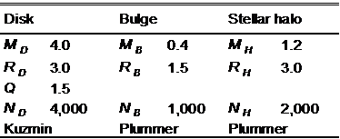
Table 5‑4: The Milky Way galaxy model G1.
In this system of units is the timestep equal to
![]() and the overall simulation
with 150,000 timesteps covers more than
and the overall simulation
with 150,000 timesteps covers more than ![]() .
.
|
|
|
|
|
Start |
1 billion years |
2 billion years |
|
|
|
|
|
|
|
|
|
3 billion years |
4 billion years |
5 billion years |
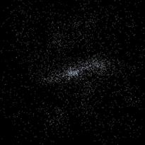
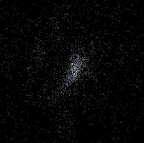
Figure 5–26: The evolution of the Milky Way galaxy G1 composite model in the xy plane.
|
|
|
|
|
Start |
1 billion years |
2 billion years |
|
|
|
|
|
|
|
|
|
3 billion years |
4 billion years |
5 billion years |
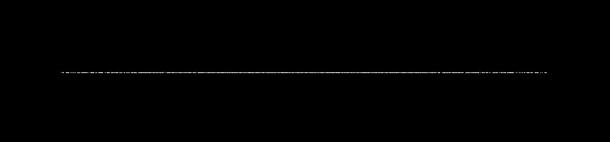
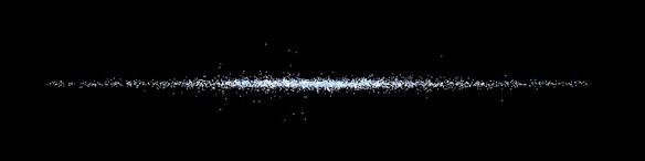
Figure 5–27: The evolution of the Milky Way galaxy G1 composite model in yz plane.
Milky Way with dark matter halo
In the Milky Way galaxy model G2, we will add the isothermal dark-matter halo component. Our galaxy is probably contained in the halo of dark matter particles with radius nearly 250 kpc that is about 20 times more massive than visible parts of Galaxy, leading to luminous-to-dark ratios of 1:20.
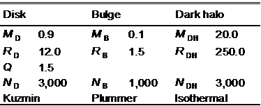
Table 5‑5: Milky Way galaxy model G2.
Simulation parameters and units are the same as
in the simulation of G1 model. The timestep is equal to
![]() and the overall simulation
with 150,000 timesteps covers more than
and the overall simulation
with 150,000 timesteps covers more than ![]() .
.
In Chapter 5, we have shown how to create a computer model of a galaxy in order to study galaxy dynamics. We found that the construction of galaxy in a controllable way is difficult. Due to immense complexity, all models are very artificial in comparison to real galaxies. In spite of that, the initial density distribution function of models are in good agreement with observations of real galaxies. The galaxy models created were single or multicomponent systems in stable dynamical equilibrium.
Initial conditions were generated as follows. Specifying the mass density distribution function, we first calculate the model’s cumulative mass distribution function and corresponding gravitational potential. Then the mass density distribution function is expressed as a function of gravitational potential. The phase-space distribution function is calculated on the fly using a numerical formulation of Eddington’s formula. Once the phase-space distribution function has been calculated, one can start to randomly sample particles from the distribution function. If the use of another mass density profile is requested, all that is necessary, is to override a virtual function “rho” according to the chosen mass density profile. Through this approach, many kinds of models may be constructed. Models created in this way are quickly getting into equilibrium.
We created realizations of an elliptical galaxy from various spherical models. The spherical models were in equilibrium from the beginning. We have created disk models that showed continuous evolution. We saw that dynamically cold disk without a dark halo spontaneously formed features resembling galactic bar and spiral arms. It has been shown that a self-gravitating disk system is unstable unless a certain velocity dispersion and dark halo were included. All models were evolved for more than 1 billion years and movies from all computations were produced.