“A picture is worth a thousand words.”
“An animation is worth a million words.”
8
Simulation Software
In this chapter, we will present the main features of simulation programs and how to use them.
This thesis was written in the department of physics, so I wanted to be clear as much as it was possible in a computational side of the thesis. Therefore, I decided not to use a massively parallel implementation as I did in previous work (Schwarzmeier, 2004). My source codes are written in C++ computer language, because it bears both qualities that I require on the computer language and compiler for the galaxy dynamics educational-research work: portability (people in education usually work in Microsoft Windows environment, while people in research on Linux workstations) and high processing speed of compiled code[64]. In any case, anyone is free to choose the favorite programming language and platform according to her or his choice, while guided by a physical description in the text and numerical description in the source codes.
All source codes[65] are written in ISO/ANSI Standard C++ with Standard C++ library and should compile with any C++ compiler conforming to these standards. I used freely available Microsoft Visual C++ 2005 Express Edition[66] for the Microsoft Windows platform and GNU C++[67] for the Linux platform. The source codes utilize two widely used third-party libraries: GNU Scientific Library (GSL)[68] and LIBXML2[69]. After unpacking the code, it must be compiled. Solutions and makefiles are in the /amon/_make/ and /ics/_make/ subdirectories. Hopefully, the compilation should be successful.
The code created for this thesis may be used by a student in two ways. The code can be used as a finished program that can be executed with command-line parameters in order to create galaxy models and evolve them. The second and more desirable way to use this software is to extend it. I have used an object-oriented design that enables the extensibility and reuse of existing simulation classes through the addition of new physics without the need to rewrite the original code. A student, who makes extensions to the existing simulation code, will reach the top of the educational pyramid presented in Chapter 2: New Pedagogy.
All calculation using the AMON-2 (Astronomical Modeling with N-bodies) code are run using the executable amon-main in the /amon/bin/ subdirectory, but you will need different input files to tell the code to do different things. We begin with a description of routines used to start a new calculation from scratch.
Generator of Initial Conditions (GENICS) is, in fact, a set of programs and classes located in the /ics/ directory. Executables should be located in the /ics/bin subdirectory after the successful compilation. All executables are console (command line) applications[70].
8.2.1 Spherical galaxies
Let us suppose that we want to create a spherical galaxy called “Model A” consisting of 5,000 bodies with the Hernquist’s distribution function. It can be done by executing the file ics-spheric-main in the command-line window of the operating system as follows
> ics-spheric-main h model_A 5000
The first switch behind the executable name can be h (Hernquist), p (Plummer), j (Jaffe), t (Isothermal) or u (Uniform). The ics-spheric-main program will generate two files in the current directory: model_A.xml and model_A_ics.bin. The file model_A.xml contains XML (Extensible Markup Language)[71] description of the simulation binary file model_A_ics.bin. The simulation binary file will contain the generated simulation data of Hernquist’s model, i.e. masses, positions and velocities of individual bodies.
To verify the validity of numerically calculated functions, it is useful to produce their plots. It can be done by plugging a p (plot) parameter at the end of the command line:
> ics-spheric-main h model_A 5000 p
With the p parameter, the program will create a series of files with txt extension that are suitable for plotting with gnuplot[72]. When Microsoft Excel is installed on a computer, ics-spheric-main also creates a new instance of Microsoft Excel through the Microsoft Windows’ Component Object Model (COM), inserts tabulated values of numerically calculated functions into an Excel sheet and automatically generates an Excel chart for each of these functions.
8.2.2 Disk galaxies
The generation of disk (flat) models can be done in a similar way. Let us suppose that we want to create a realization of Kuzmin’s model called “Disk A” with 6,000 bodies and plot functions numerically calculated by the program:
> ics-flat-main u disk_A 6000 p
For that purpose, we have used ics-flat-main executable that recognizes the following models: u (Kuzmin), k (Kepler), e (Exponential). Remaining parameters are the same as for the generator of spherical models.
8.2.3 Rotation
Every galaxy created by the GENICS can be optionally rotated. E. g., let us suppose that we make preparations for the collision of counter-rotating disks. Disks are generated by the ics-flat-main in the xy plane. So we must rotate such a disk around the y-axis by 180 degrees to obtain the desired counter-rotation:
> ics-rotate-main disk_A.xml disk_B 0.0 180.0 0.0
This essentially says to the ics-rotate-main program: take a galaxy described by the disk_A.xml file, transform it by rotations of 0.0 degrees about the x-axis, 180.0 degrees about the y-axis and 0.0 degrees about the z-axis and save it to disk_B binary and XML files.
8.2.4 Conversion of units
Now imagine that we want rescale units of a generated galaxy, i.e., change its gravitational constant, scale length and mass. We can do that by executing the following command
> ics-units-convertor-main model_A.xml model_B 1.0 0.1 0.001
This command will execute ics-units-convertor-main that will read a galaxy described by the model_A.xml file and rescale it, while leaving the gravitational constant the same (1.0), multiply its scale length with 0.1 and its mass unit with 0.001.
8.2.5 Direct collision
To set galaxies on a direct collision course, the ics-encounter-main program with the d parameter must be evoked. Consider as an example the following command-line:
> ics-encounter-main d galaxy_A.xml galaxy_B.xml collision 10.0 0.5 0.1
The listed command will set galaxies described by the galaxy_A.xml (central galaxy) and galaxy_B.xml (companion galaxy) files on the direct collision course with the z-axis distance equal to 10.0, z-velocity equal to 0.5 and x-axis shift equal to 0.1. This collisional configuration will be written to collision.xml and collision_ics.bin files.
8.2.6 Keplerian encounter
Galaxies can be set on Keplerian orbit as follows
> ics-encounter-main k galaxy_A.xml galaxy_B.xml collision 10.0 0.8 25.0
Notice that we have changed the first parameter of ics-encounter-main to k (Keplerian). The meaning of numerical parameters is now following: a semi-major axis is equal to 10.0, numerical eccentricity equals to 0.8 and true anomaly to 25 degrees.
8.2.7 Extensibility of GENICS
Not all features of the GENICS, however, are accessible from the command-line. Anyone can come with a new mass density distribution function of a galaxy and try to test its evolution. This can be simply done through deriving a descendant class from the CSphericalModel class and overriding the rho virtual function as is done, for example, in the Hernquist’s model:
#include "sphericalmodel.h"
// derive descendant class
class CHernquistModel: public CSphericalModel
{
public:
CHernquistModel()
{
m_name = "HernquistModel";
}
protected:
// override with a new mass density distribution function
virtual double rho( double r )
{
if (r == 0) return 0;
return ( m_totalMass / ( 2.0 * M_PI * pow(m_a,3) ) ) *
( ( pow( m_a, 4 ) / ( r * pow( r + m_a, 3) ) ));
}
};
A full hierarchy chart of GENICS can be seen on Figure 8–1.
AMON-2 is a tree N-body simulation code for evolution of three-dimensional self-gravitating collisionless systems. It is based on the Barnes-Hut algorithm. Executable amon-main should be located in the /amon/bin subdirectory after a successful compilation.
Syntax is following:
amon-main [algorithm] [input_file] [timesteps] [theta] [epsilon]
[group_size] [timestep] [gconst]
Parameters:
algorithm
Specifies which algorithm will be used: b Barnes-Hut, d direct (brute-force) calculation.
input_file
Specifies the simulation XML file.
timesteps
A total number of timesteps.
theta
Parameter ![]() from the
Barnes-Hut algorithm.
from the
Barnes-Hut algorithm.
epsilon
Gravitational softening ![]() .
.
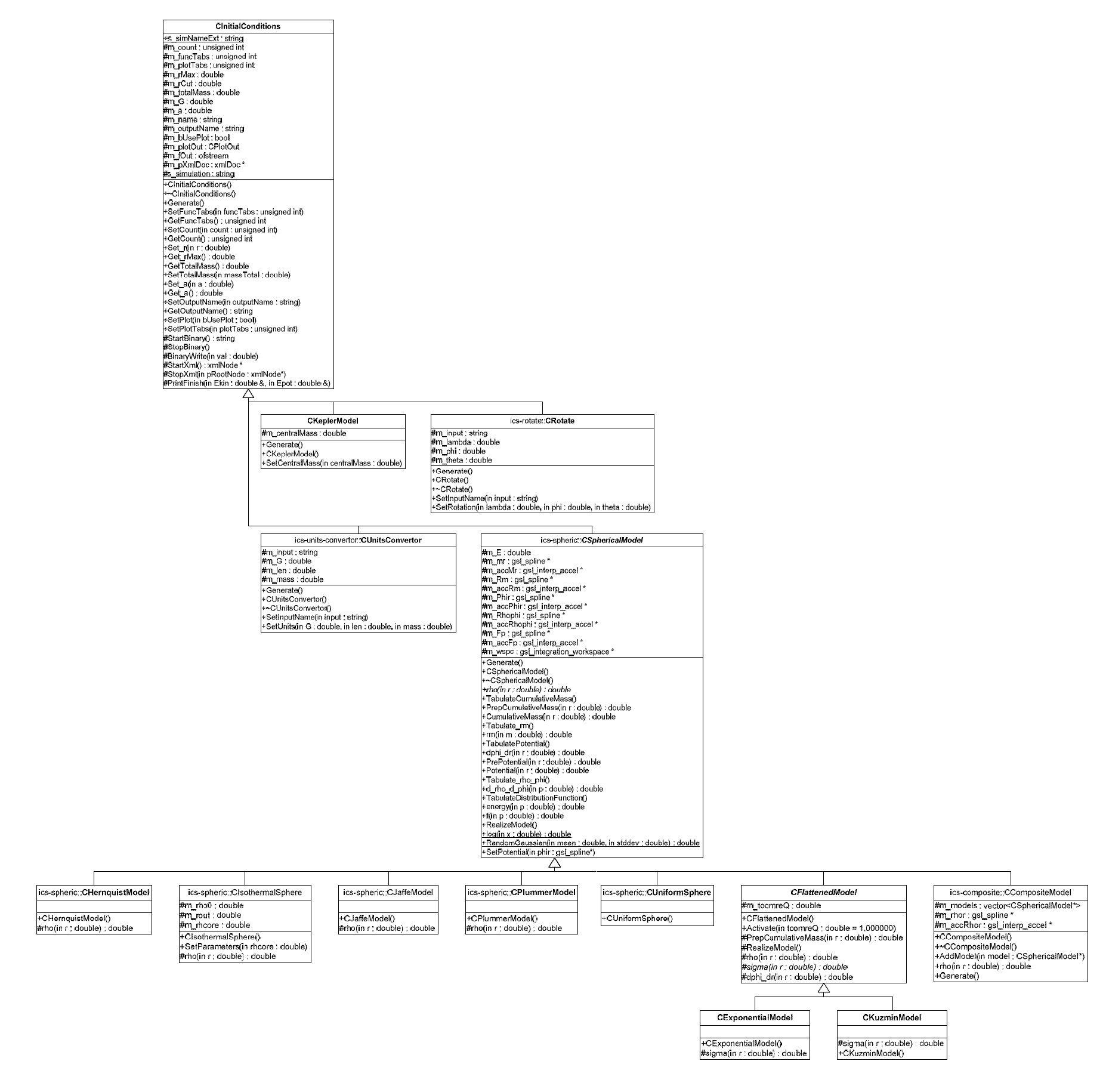 Figure 8–1: UML
(Unified Modeling Language) diagram of the Generator of Initial Conditions
(GENICS).
Figure 8–1: UML
(Unified Modeling Language) diagram of the Generator of Initial Conditions
(GENICS).